Welcome back!
It’s been quite a while since I’ve updated this blog, sorry about that. But don’t worry, I’m still working on the Immortal! In fact I have several things to talk about today.
First off:

I can draw tiles!
But before I get into the main part of this post, I wanted to also mention that my branch for The Immortal has been merged into the main ScummVM repo, and as a result my ProDOS disk reading code has been moved into common! This is great, as now other engines can utilize it for reading ProDOS disks in the future.
Alright, tile drawing is a complicated thing so buckle up, as this will be a long one.

Last time on “This code is complicated”
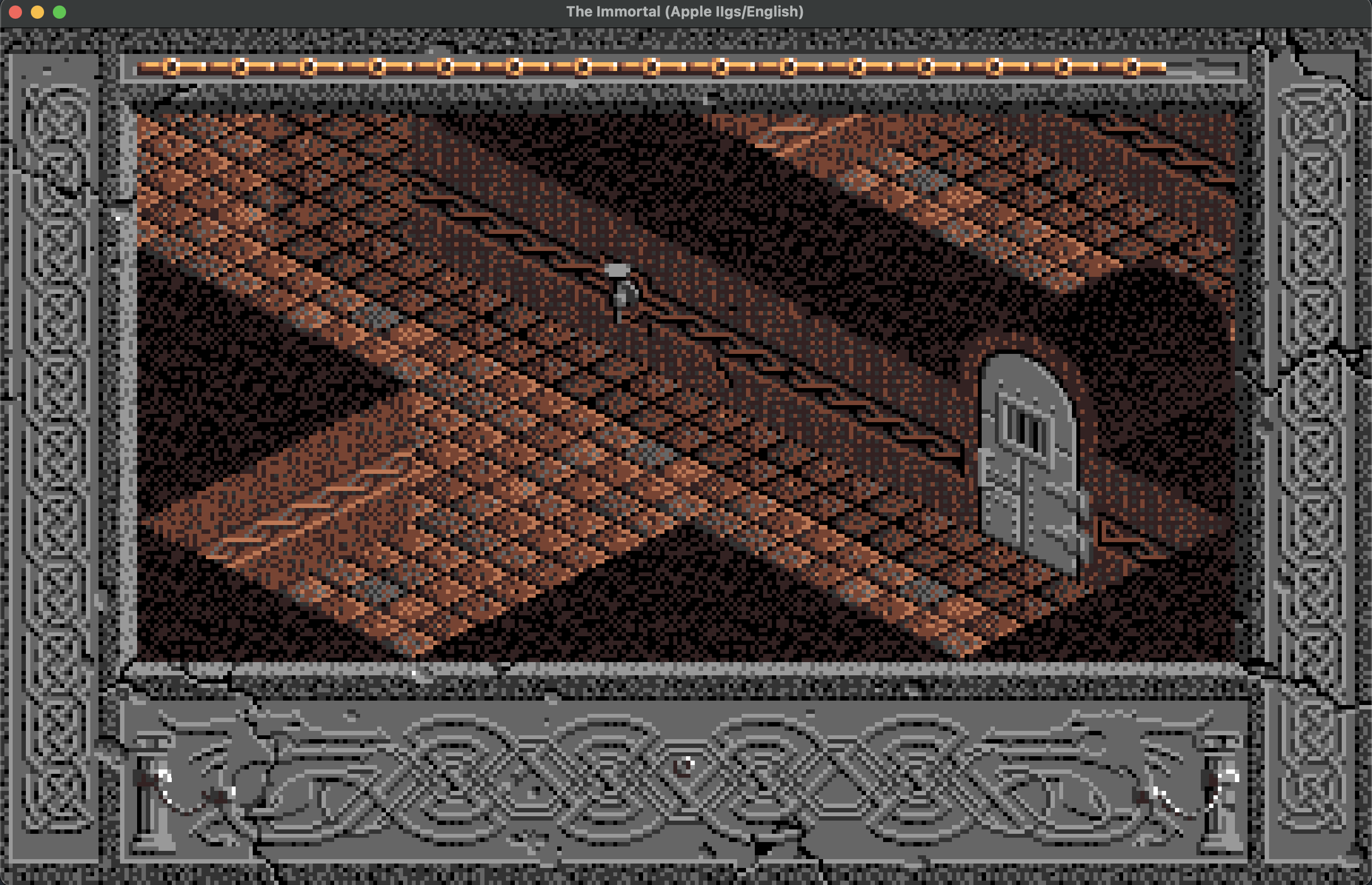
Now, when I left off last time, I was saying that the next big thing to deal with was reading .CNM and .UNV files, because these seemed to contain the level data, graphics data, and universe properties for a given level. At this point, the flow of logic has gone like this: Main game loop -> logic() -> restartLogic() -> fromOldGame() (this is where the title strings get drawn) -> levelNew() (this is where it loads all the properties for the level including the ‘story’) -> loadMazeGfx() -> loadUniv(). At this point, it was clear that the game had loaded the properties for items, enemies, objects, etc. and was now going to load the actual graphics data itself. However, it wasn’t clear exactly what was being loaded at what point, or how any of it worked. What I knew, was that you had two files per level, a .CNM and a .UNV. One was much bigger than the other (unv), so it was likely that one contained the gfx. But where it got complicated, was with what a CNM was, and how it relates to all the other references to CNM and CBM and various other initialisms throughout the source. When translating various kernal functions, I encountered some of these names in reference to building the ‘universe’, but there was never enough information to make out exactly what the structure was. And without the structure, it would be hard to work with any of it. I also knew at this point that the file DrawChr was clearly responsible for drawing the background tiles. However the way it did so, was an absolute mystery to me. I want to give a sense of how complicated the assembly code looks for it, so here is an example of one of the many, many complex tables used by the drawing routines:
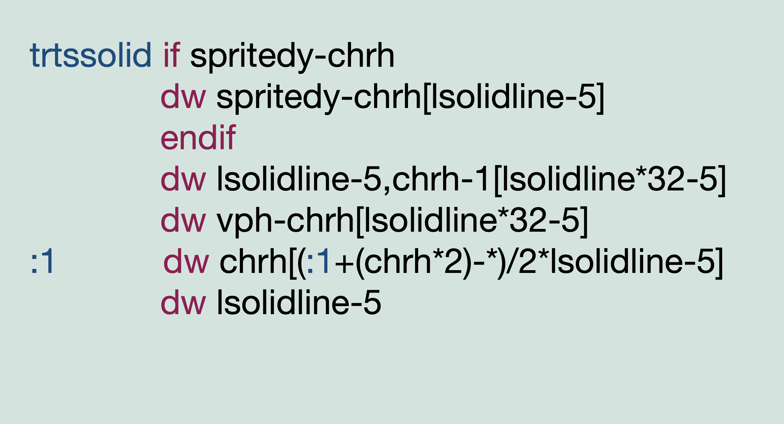
You may be looking at this table like

Which is about how I felt as well. This table has elements like ‘chrh[(:1+(chrh*2)-*)/2*lsolidline-5]’, and is not even the most difficult to read table there (the really hard to read ones include many magic numbers that require a lot of running around in the source code trying to find what it corresponds to). But even this one needs to be broken down bit by bit to try and determine what any of it means. For example, you need to know what [] means in the context of this compiler. Similarly, what * means when it is not being used as a multiplication (it can also mean the cursor position). You also need to find what lsolidline is, and why it’s subtracting 5, why chrh is being multiplied by 2, etc. And that’s just one part of the table. So going into this without knowing how any of these tables are used, requires quite a bit of time dedicated just to untangling the web of references and data. On top of that, let’s take a look at a part of one routine that is used by the main routine that will be important for all of this (with any comments removed and some terms simplified for this example):
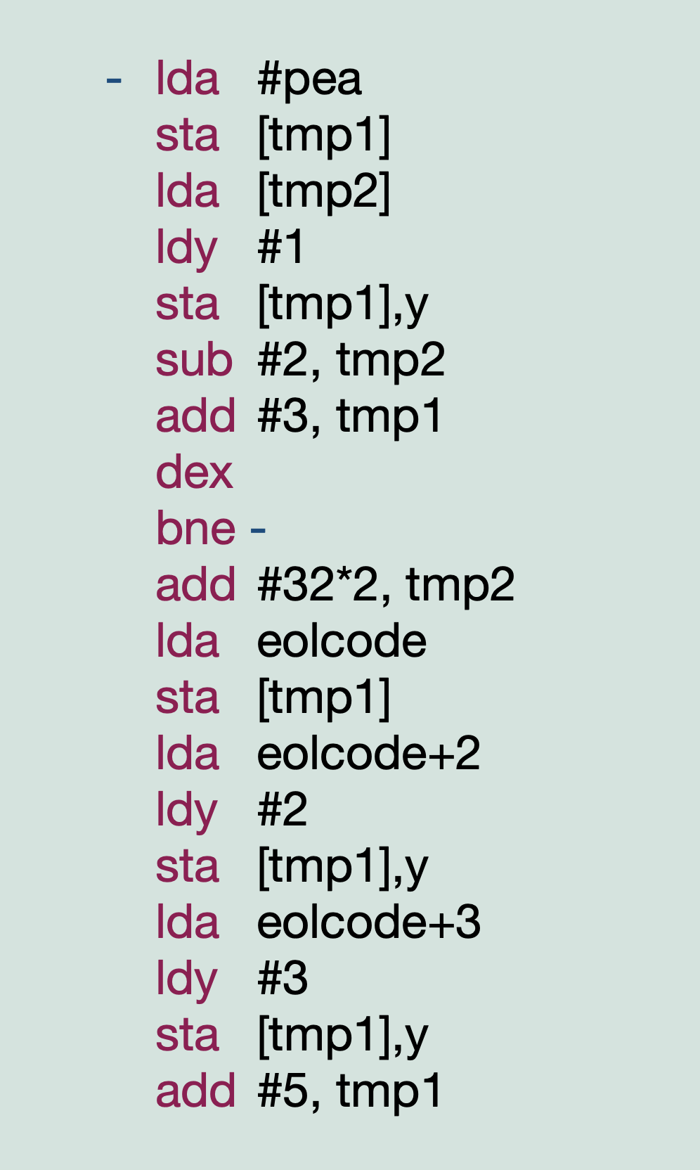
At first glance, this doesn’t seem so complicated. We can presumably replace tmp1 and tmp2 in our head with what we know they contain as the routine is run (they are loaded and stored to indirectly, so we know they contain addresses of some kind), and then it seems like a fairly simple loop. Except…there’s that #pea and something called ‘eolcode’. These are a little odd, so we need to take a better look at them. Now keeping in mind that we don’t know at this point what the exact purpose of this routine is, seeing #pea is a bit surprising. The reason is that, true to it’s label, pea is a reference to a single byte, which happens to be the byte representation of the opcode, you guessed it, PEA. So why is this surprising? Because no matter what address is in tmp1, the game is writing the byte code for an operation into that memory location. Regardless of the rest of the code, this is at the very least a weird thing to see. It’s writing code into memory that will presumably be run from that memory later on. And then we get to eolcode, which is a reference to a small block of code. Now with this information we can at least put together that this routine is writing some kind of set of operations (it performs a loop that continuously writes at least a PEA operation), followed by a block of predefined code (each byte of the eolcode block is written into the same place as the PEA). Now, this is especially odd given the fact that we are apparently dealing with loading graphics data right now. So why is there a routine which is fundamental to the system, writing code instead of graphics data into memory? To add to the confusion, there are several other routines that are called in a similar way, and contain code that looks vaguely similar, but much more complex (multiple larger loops that store more operations than just PEA).
Now we’re caught up
So by this point, we are looking at a routine (mungeCBM()) which seems to take the decompressed gfx data, the decompressed CNM, and the logical CNM, and performs some kind of magic where it dynamically writes out code into memory instead of graphics data, to create a new data structure (this is what the munge refers to, it combines and permanently alters the data of these structures to create a new one) comprised of a few arrays of data, called Solid, Left, Right, and Draw. The question at this point was, where do I even start for untangling this? There is no clear definition of CNM, nor is there any explanation about the type of data stored in the CBM. The routines involved seem to dynamically write code where you would expect graphics data to be, and the drawing functions reference extremely complex tables with no explanation about their purpose or how they function. And to top it all off, the code that gets written into memory seems to utilize this PEA operation extensively, an operation that I had come to know as the ‘change data bank or return address’ operator. That’s certainly an important part of many routines, but why is it used so extensively in the dynamically generated ones? And how is the actual graphics data read? And what even is the graphics data? Is it bitplane, or linear, or something more proprietary? One thing we do know at this point, is that the author of this code is the same person that wrote the sprite handling code, which is a genius bit of very complicated assembly designed around saving processing time when moving pixel data, so nothing is off the table when it comes to how this tile rendering code could work.
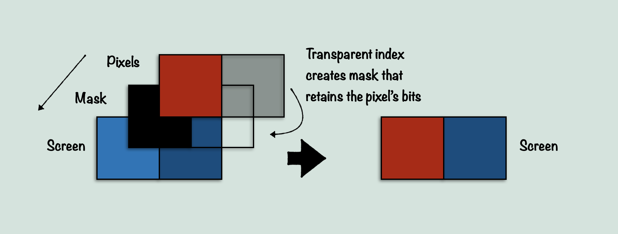
Speaking of which, let’s talk briefly about sprites. I mentioned in my sprite explanation that there was something else the sprite code did that was very interesting, but that I was likely to talk about it later on when I got to tiles, since it seemed to do something similar. This was kind of accurate, although I had no idea what it would end up actually being. As I explained in that earlier post, sprites do a few notable things to save performance. One of them is to use a large table of masking values to automatically determine how transparency will affect the pixels of a sprite. Sprites are stored as two pixels per byte, 4bpp packed pixels in other words. This is the same way the screen buffer stores pixels. So ideally, you would want to store the pixels directly to the screen buffer so that you can load 2 pixels per byte in one operation, and store them to the screen in the next operation. However this doesn’t work with transparency. If one of the two pixels is transparent (an index value of 0), then we need to not store that value to the screen, overwriting the screen pixel. Instead we want to preserve the screen pixel for just that one pixel. Normally, to do this you might extract each pixel, check if it’s transparent, and if it is, then don’t store it, otherwise store it. This is fine, but costly. LDA $pixels : AND #$0F : BEQ + just to check transparency per pixel takes quite a few cycles when you add up the number of times you have to do it per sprite per frame. So instead, The Immortal uses a system where it has a large masking table that contains an entry for every possible value from 0 – 255 (FF). This way, you can have a mask for any time the pixels include a 0. 10 for example, could get you a mask of 0F, which will make sure to grab the pixel value of the screen pixel. In this way, we can handle both pixels at once including transparency, at a relatively small cost. LDA $screen : AND $masktable, pixels : ORA $pixels. This way no extraction has to happen, and branching either (this is simplifying the entire process, but I hope the point is clear). I used this diagram to show the idea:
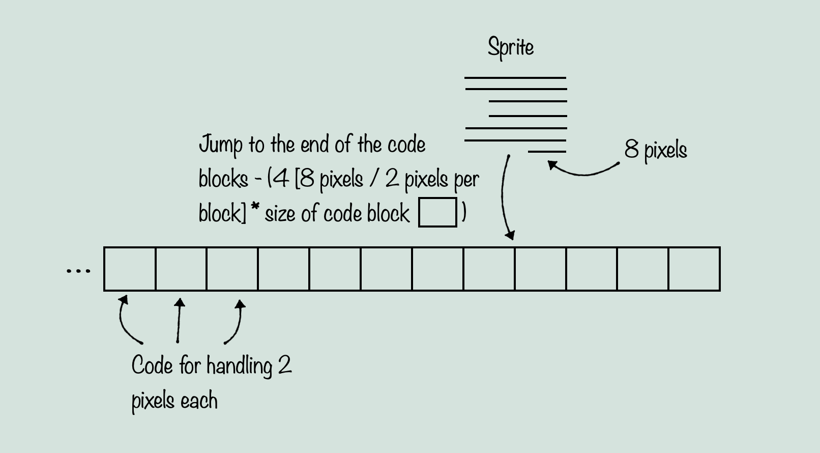
But the other thing that is noteworthy about sprites, is how the code for these pixel handling is executed in the first place. This is where it gets interesting, because it takes the idea of unrolling a loop to a whole new level. When you think about loading and storing pixels from graphics data into the screen buffer, you probably imagine a loop of some kind. But loops are slow, relative to how many times we need to grab pixel data for sprites per frame. So instead, what The Immortal does, is store a giant, unrolled loop that covers one full scanline of the largest size a sprite can be. So if a sprite’s maximum size were for example, 32 pixels, the code would be a series of that pixel handling code, 32 times in a row. Now this is fine, except there are sprites which do not use the full width, and instead have much smaller numbers of pixels, so you don’t want those sprites to waste processing on pixels they aren’t using. This is where the neat trick comes in. The Immortal treats the entire block of code as a large array, and then by using self-modifying code it redirects a JMP statement to the location of the start of just the number of pixels needed for the width being drawn. So if you have a row of 8 pixels to draw in the sprite on a particular line, it will jump to the end of the code block, minus 8 * the size of a single pixel handling code block. This way, there are no branching statements, no indexes, and no need to slow the pixel handling down by extracting individual pixels. It’s a clever, efficient way to draw pixels. The reason I mention this, is because we’re about to see an even more clever way to draw pixels to the screen. But first, here’s a diagram of what I just explained:
Alright, getting back to where I was when originally trying to translate this system. I didn’t know how the tile system worked (how big are tiles, how are they stored, how are the pixels themselves stored, where in memory are they going, how are they drawn from, etc.), but it seemed to me that the UNV file contained the CNM and the CBM, being some kind of grid representing the map, and some form of bitmap either containing the full map or a tile system of some kind. This was correct, but how they worked would turn out to be a very complicated and different thing to parse. So to start things off, let’s finally talk about the CNM and the UNV.
The CNM

UNV pretty clearly stands for Universe, but what does CNM stand for? That’s a great question that took me a long time to figure out. Don’t worry, I’ll save you the time scouring source files and staring at assembly code, it stands for Character Number Map, which doesn’t really tell you much about it, but trust me it was a huge relief to discover this name. So now we know that there is a Character Number Map, a Logical CNM, and what can be surmised to be a Character Bit Map. What exactly is a character? That remains to be seen, but we know we have graphics data in one place, and some kind of reference to that data in another place. So far this is looking similar to tile tables that you might find in a console game. A data structure that references individual 8×8 pixel tiles of graphics data, so that the graphics only needs to include one copy of any given 8×8 pixel tile. The tile table constructs larger tiles out of those, and then a level data structure can reference the tile table, to produce the level data. Well, it’s a little more involved in our case, but that is still generally the idea. You have graphics data that is used more than once to construct the level data, however, true to it’s name, the important routine here ‘munges’ a lot of this data together. We start with just three things, the Logical CNM, the CNM, and the CBM, and we end up with one data structure that sort of contains all of them combined. Now, I won’t walk through the entire process of deciphering how the system works, because it will probably take long enough just to explain the system as it is. So to explain how the system works, we can start out with loadUniv(), which takes the two files, slightly modifies the logical CNM, extracts the universe property data out of the UNV, and then decompresses the CNM and CBM out of the UNV. It then calls mungeCBM(), and this is where the important stuff happens. When we enter that routine, this is what we have:
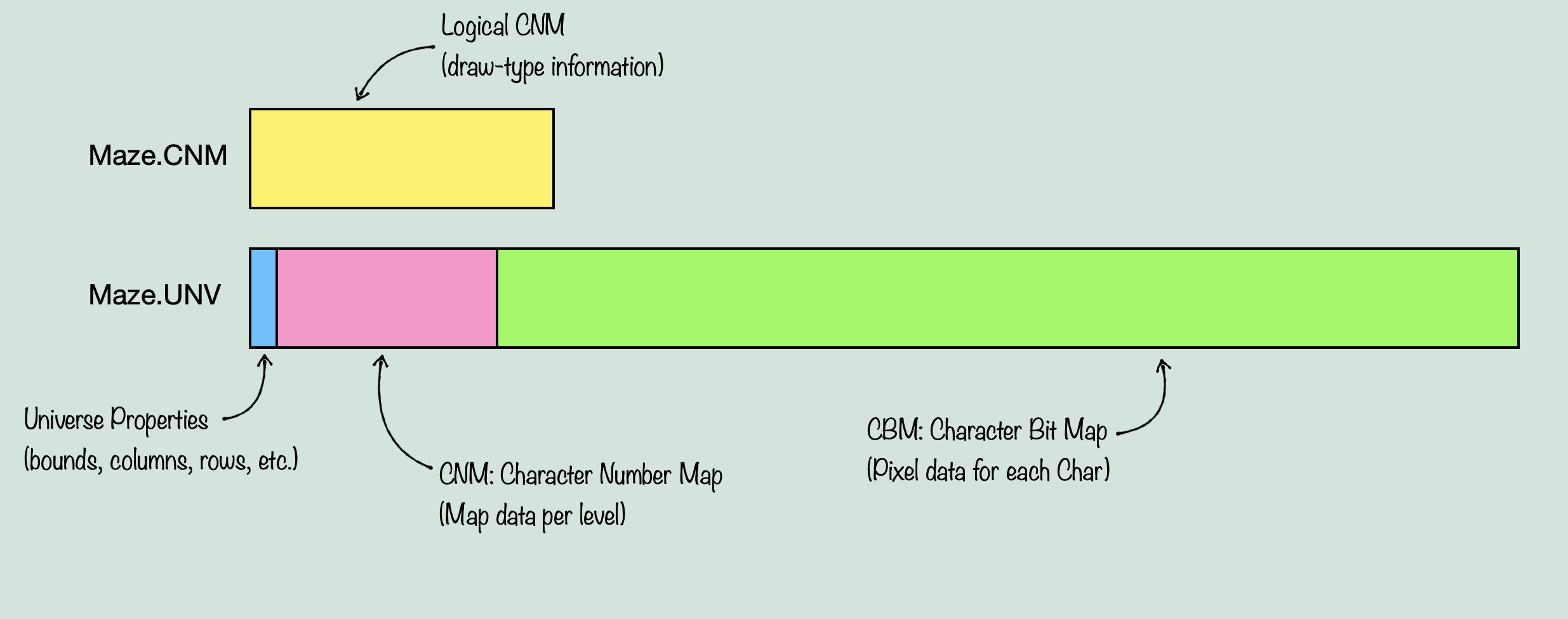
The first step is to prepare the new data structure. This will consist of the CNM, followed by an array the size of the total number of characters in the graphics data, called Solid. Then another for Left, and one more for Right. After this, is an array of unspecified length, called Draw. Together, this data can be used to draw the entire map. Before we munge together this new data structure, we have to know what the component parts are. The CNM is a map of every ‘cell’ that makes up the level map. This is usually (possibly always?) 0x500 bytes in size, with each word representing one cell, for a total of 640 cells. Each cell has a number which references a ‘chr’ in the CBM. Each ‘chr’ is a chunk of graphics data that makes up part of the visible screen. Now chr is used in several different ways throughout the source, but in this case, it refers to a 64×32 pixel chunk of graphics data. As such, you can fit 4×4 chrs on screen at once, filling up the viewport (256×128 pixels). The Logical CNM on the other hand, contains an entry for each cell of the CNM, and it has a different kind of purpose. It doesn’t directly reference the CNM or CBM, but is instead indexed with the same ‘cell’ index as the CNM, and the data it does have references a table of values that will determine something called ‘corners’. With this, we can now start to understand the purpose of the Left and Right arrays. The idea here, is that every chr in the CBM might not need to draw it’s entire data for a given tile. This is because of the way layering works in The Immortal. The Apple IIGS, unlike consoles of the time, did not have distinct, hardware based layers. Instead, sprites, backgrounds, and foregrounds all had to be drawn individually in the software. So if you wanted sprites to draw over the background, you had to handle transparency. If you wanted a foreground in front of sprites and the background? Now you have to devise a system for how tiles can overlap each other without wasting too much processing on drawing pixels over other pixels. The way it might work on a console, is that a given tile might be assigned a layer priority. These layer priorities then tell the hardware when to draw them as it combines the layers together to produce a final image. Sprites could have their own priority system, and then the sprite layer itself could be assigned priority relative to the other layers. Using dedicated hardware in a PPU, you could imagine a system that handles layer mixing efficiently and without too much input from the software. But, and this will be important later, the Apple IIGS didn’t have a PPU. Instead, this kind of system had to be designed efficiently in the game software itself. So what was The Immortal’s solution? To draw the game in three stages. First, you draw all tiles that will be behind sprites, objects, and the foreground. These are the background tiles. Then, you sort the objects and sprites based on priority levels, and draw them on top of the background, taking into account transparency. Finally, The foreground tiles get drawn on top of the sprites and background (not having to deal with transparency, but we’ll get to that).
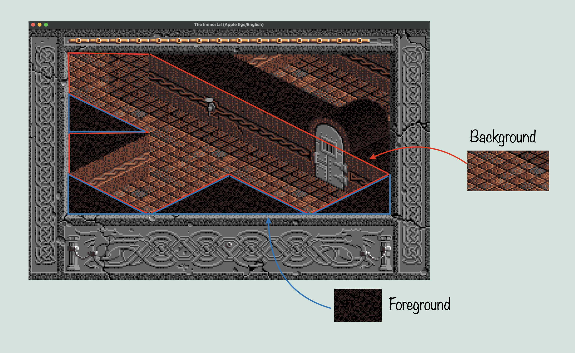
Sounds simple enough. Except that there is something else going on. The chrs are all 64×32 pixels, which means that unless you package them similar to sprites where you have distinct scan lines instead of a standard bitmap, you will need to store separate versions of tiles that only include the foreground, and not the background. This could be done in the graphics data itself, but for any number of reasons, it was not. Instead, this is where Left/Right come in. When the chrs are being munged (which will be explained shortly), the logical CNM is used to determine whether a given tile needs to have another version of itself, with some portion removed so as to let it function as a foreground. This can be done with any tile, and is determined by looking at every chr that is used in the map with the CNM, and if it is used in a way that requires foreground transparency, it creates a separate tile, which will then be referenced by either right or left, depending on which side of the tile the corner is that will be transparent. Remember that this game is isometric, which means our transparency is based on corners, not quadrants. The separate tile it creates, it put together with a special version of that routine I showed part of earlier, but instead of using all the graphics data, it only looks at pixels up to a diagonal line across the tile, depending on the corner. Solid, on the other hand, simply uses the entire chr’s graphics data, creating a standard chr. By the end, CNM contains references to chrs, which are used to now index one of Solid, Left, or Right, which contain references to the actual chr graphics data, or the modified chr data. So our new data structure looks like this:
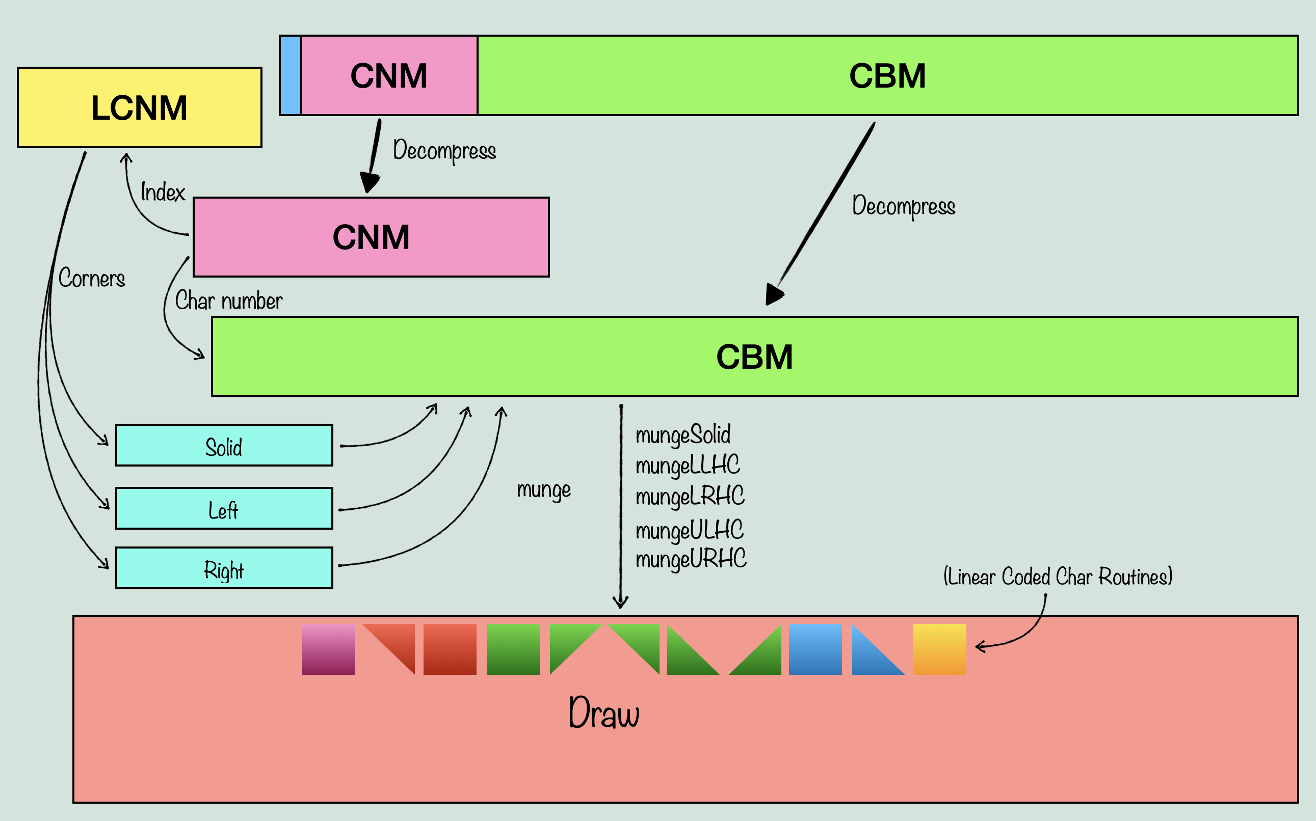
Hm, what are ‘linear coded char routines’ referenced in the diagram? Well, that’s the next, and most interesting topic.
So, the big question from before was what that routine was doing writing code instead of graphics data. Well, let’s get into it.
To start, let’s talk about why ‘munge’ is an appropriate name. Munging basically refers to changing/manipulating/converting data from one format into another, usually permanently. In this case, it is referring to how it takes graphics data as a set of pixels, and converts it into a set of operations that makes up a dynamically generated routine. This routine is quite simple, but putting it together from the code is much less so. The end result is that by using the munge routines, we can take pixel data and turn it into routines that store the direct pixel data from the CBM into the screen buffer, move down after each scanline, and end when there are no more pixels. In the case of the corner routines, they make sure to only create operations on pixels that are part of the visible corners of the tile. This means that when this code is executed, it won’t have to worry about transparency, because it is only moving pixels that are visible. So as long as the drawing routine knows where to place those pixels, it will never overwrite pixels it shouldn’t. This also solves another problem, transparency in layers generally. Instead of the foreground simply overwriting pixels in the background, we can use these corner tiles to draw only the background pixels that will not be covered by foreground pixels, and only draw foreground pixels that aren’t overwriting background ones. This way the only pixels that get drawn over, are the sprites.
Pixels -> Routines
Okay, so it turns the pixel data into routines, that means we take $1234 and turn it into LDA $1234 : STA $screen,x : INX #2, right? Not quite. Remember how it seemed to only store one operation, PEA, before the end of line code? Well, this is the really interesting, and extremely confusing to decipher, aspect to these routines. They really do only use a single operation, PEA. So first then, what is PEA and why is this interesting in the first place? PEA stands for Push Effective Address, and has a particular purpose in 65816 assembly, to push an address onto the stack. What that means, typically, is that you can use it to change what bank you’re loading data from, or what address will be returned to after a jump instruction. This is because the argument it accepts is a direct word, two bytes. It is similar to other stack pushing operations, except that it doesn’t push a register, it pushes a direct address, so that software can manually change addresses used in the stack. So then, how does that relate to our graphics movement? Well although a loop, or even an unrolled loop, of loads and stores is effective, it is costly. Remember the sprite drawing routine, which switched out the branching and extra loading for a table to make it more efficient. Similar to that, we need the most efficient method of moving data here, because we are moving even more pixels of data than we were with the sprites. So if LDA : STA is costly, what other option do we have? You have to somehow get the graphics data, and then store it to the screen buffer. Then, since we don’t know the exact position in the screen buffer to store to when converting the graphics data, we need to increment the destination as well. Here is where PEA comes in and does something magical. PEA is typically used for moving addresses, but as ‘Programming the 65816’ notes, “Although the mnemonic suggests that the sixteen-bit value pushed on the stack be considered an address, the instruction may also be considered a “push sixteen-bit immediate data” instruction, although the syntax of immediate addressing is not used” Which is to say, although the syntax is not the same, you can technically consider PEA the same as LDA #$value : PHA, as it takes a direct 16 bit value and moves it to the stack. Since we are converting graphics data, and not loading it, we would love to be able to simply turn every two bytes of pixel data into a PEA $pixels. However, you may be wondering, how does that actually help us, if it’s storing it to the stack? We need it to get to the screen buffer. Well, this is genius of it all. What if the stack, weren’t the stack? What if, instead of the stack pointing to an array of addresses and values in memory, it could be pointed instead to the screen buffer itself? Well then, pushing to the stack would instead push to the screen buffer, which happens to be exactly where we want to move data. But then we still have one problem, the destination has to be incremented, because we don’t know the exact position when converting the data. Ah, and once again the genius of this method is revealed. The stack increments itself (or rather, decrements, but that’s not the point here. The pixel data is stored and written back to front). The stack has to handle it’s own incrementing already, because that’s how stack operations function. This means, if you were to push directly to the screen buffer and the CPU thought the screen buffer was the stack, then it would automatically increment the position, as if you had manually performed the INX #2 needed. By tricking the CPU into thinking you’re working with a large stack, you are effectively bypassing both the load operation, and the increment operation. And in the end, you can turn LDA #$pixels : STA $screen,x : INX #2 into PEA $pixels. That alone saves about 2/3rds of the processing time per group of pixels moved. And considering we are talking about moving 4×4 chrs of 64×32 pixels each, every frame, we are talking about saving a tremendous amount of processing time. Here’s a quick diagram:
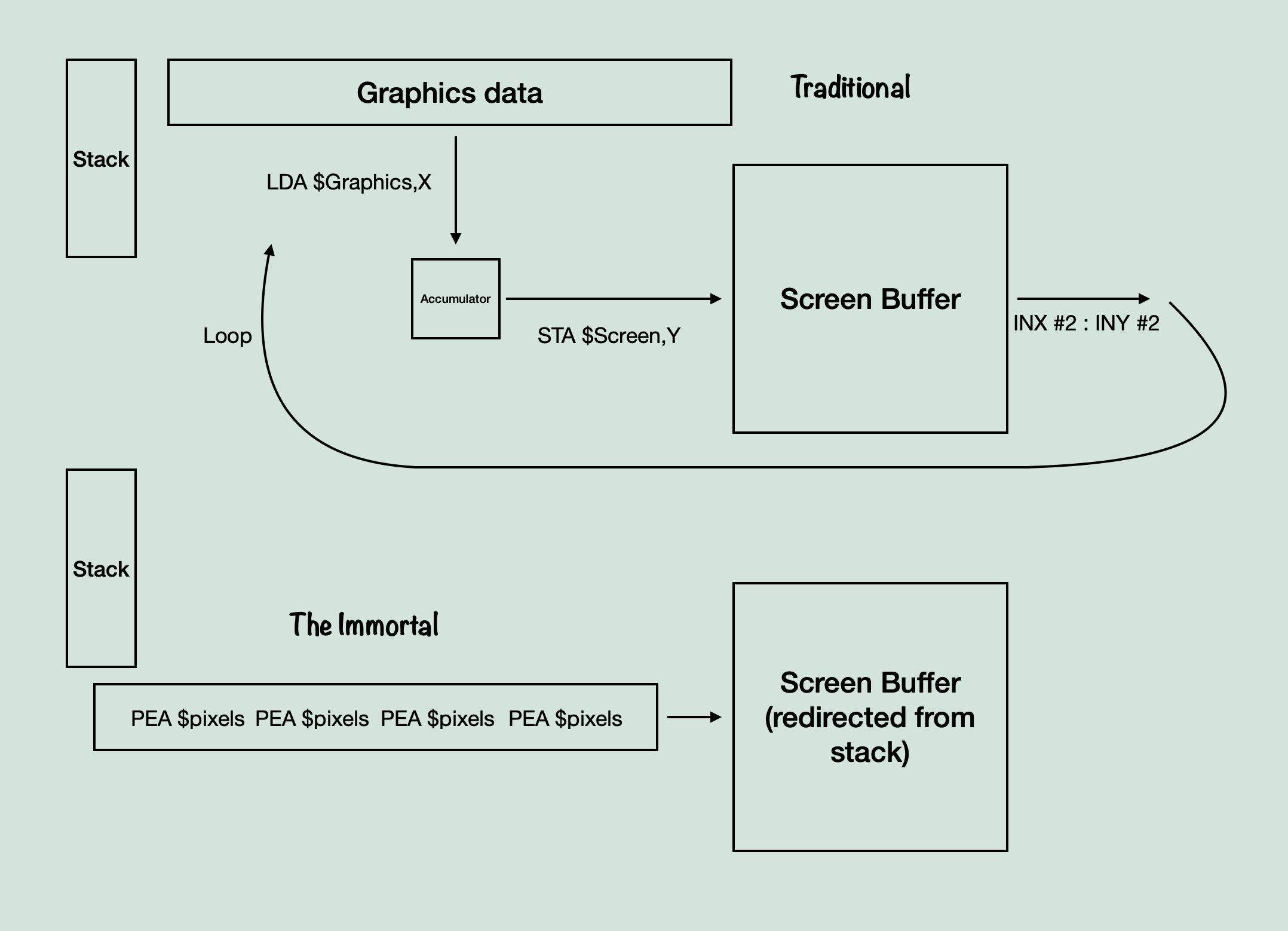
The method on the top is the most basic system, where you just load from somewhere and store to somewhere else. Presumably, other games converted graphics data into data movement operations if they needed the processing time as well, but I’ve never heard of one utilizing a PEA operation like this before.
Recap
The graphics data gets transformed into ‘linear coded chr routines’ which consist of PEA operations. These routines get referenced in Solid, Left, and Right, indexed by the CNM value thanks to the Logical CNM. When it comes time to draw the graphics, using some very complicated tables and careful addressing, we save the current stack location, point the stack to the location in the screen buffer of our tile, and then jump to the routine that represents our graphics data, which will push only the pixels it needs to and then end itself when it’s finished. No need to worry about transparency, because it only has PEA’s for the pixels that are visible, and the draw routine simply has to know where to start executing those PEA’s on the screen.
At the end of the day, this system for loading and drawing tiles saves processing time by re-purposing a particular opcode in the 65816 CPU, using a method only applicable to assembly (repointing the stack to the screen buffer), at the expense of it being very hard to follow without prior knowledge of the system’s inner workings.
End

Yes, this post is finally over, thank you for reading all about graphics and assembly, I appreciate it!
I want to apologize for the delay in getting this post out there and finally showing some more progress on the port. I definitely felt somewhat burned out after GSOC, and every time I looked into these routines, it became less clear how they worked, not more clear. But I finally understand how this odd system of graphics works, and I’m excited to get back into the translation.
Speaking of which, how on earth does this assembly translate to C++? Short answer: it doesn’t. I can’t exactly replicate the stack manipulation and execution of dynamically generated routines in memory, so instead we need to take some liberties. My version of this system is a little more simple. You still have the general structure of CNM, Solid, Right, Left, and Draw, but now they reference an index into Draw as an array where each element is a collection of scanlines, being only the size of the visible pixels. Then, when drawing the graphics the draw routine simply applies that pixel data in the same arrangement to the screen buffer. It’s not exactly the same, but I think it gets the same general logic.
Now, I didn’t go over a number of things, like chr clipping, or the process of determining what type of pixel storage it used, or some of the nitty gritty of the assembly, but I hope I conveyed how interesting and hard to decipher from the inside out this system is. It’s fascinating stuff.
Next
I may go over decompression, because I had to rewrite my old decompression functions, and the way this version of LZW works is pretty interesting.
Until that time, thanks for reading this terribly long post, and I’ll hopefully be back again soon with something shorter.